Can distributed AI nodes learn to cooperate? The Dendrite experiments
Three AI nodes, each watching one stream of market data. They’re supposed to get smarter together than apart — that’s the whole premise. I run the experiment. The collective performance is essentially identical to the individuals. Then marginally worse.
That’s not a great start. But it’s an interesting start, because the failure has a specific shape, and the shape tells you exactly what to fix. Here’s the full story, from the hypothesis through the architecture through what actually worked and why.
The idea
DENDRITE is a project I’m building to test whether you can make a useful AI system out of many small, specialised nodes instead of one large monolithic model. Each node sees a fragment of the world, does its own local inference, and communicates with other nodes through a shared representation space. The bet is that the collective network — many partial views reconciled into a consensus — can outperform any individual node.
This is a testable claim. I’m spending a few weekends finding out if it’s true.
There are five specific claims to validate, in order. This post covers the first two:
- Can a single node learn useful representations from continuous streaming data? (Can predictive coding work at all here?)
- Can multiple heterogeneous nodes align their representations and collectively outperform individuals? (Does the coordination mechanism actually help?)
The remaining three — sleep-wake cycling, active inference, pathological precision states — are for later posts.
Why cortical columns
Before running experiments, you need to decide what a “node” actually is. The design choice is a cortical column: a small neural network with internal structure loosely modelled on the six-layer organisation of the mammalian neocortex.1
The motivation is functional, not biological pedantry. The neocortex doesn’t have one region that knows everything. It has many specialised areas — visual, auditory, somatosensory, prefrontal — that each build local models of their slice of reality and then reconcile those models through long-range connections. Consciousness, if you believe the theorists, is the result of that reconciliation process. The Thousand Brains Theory (Jeff Hawkins et al.) formalises this: every cortical column is an independent world-model, and the unified perception you experience is just the consensus view. DENDRITE is asking whether you can build a scaled-down, software version of this with gradient descent.
Each column has four active components:
- Layer 4 (sensory input): Receives the raw data — price stream, volume counts, image patch, whatever this node’s job is.
- Layer 6 (reference frame): A learned position vector that tracks where in abstract state space the node thinks it currently is. Not a spatial position — more like a hypothesis about the current regime or object category. Updated each timestep by a small learned transition function. Think grid cells in the hippocampus, except the “space” being navigated is the space of possible world-states.
- Layer 2/3 (model): Binds the current input (what) with the reference frame position (where) to produce a prediction of the next observation. This is the generative model.
- Layer 5 (motor output): Stubbed for now. Will eventually drive active querying — the node choosing where to look next.
┌─────────────────────────────┐
│         COLUMN NODE         │
│                             │
│  L1  ── top-down context    │ ← predictions arrive from model node
│  L2/3 ─ model (what+where) │
│  L4  ── sensory input       │ ← your slice of the world
│  L5  ── motor (stubbed)     │
│  L6  ── reference frame     │ ← "where am I in state space?"
│                             │
│  [ACI Translator]           │ → internal state → shared space
└─────────────────────────────┘
The training signal is prediction error: the gap between what the model predicted and what actually arrived. This is predictive coding — the node is perpetually trying to predict the next observation, updating its parameters to reduce surprise. Lower average error means a better internal model. Spikes in error signal novelty or regime change.
How nodes communicate: the ACI
The Aligned Contrastive Interface is what makes a collection of nodes a network rather than a bag of individuals. Each node has a small projection network that maps its internal state to a point on a shared hypersphere — a 64-dimensional space where every vector has been L2-normalised to length 1.
internal state → Linear(→128) → ReLU → Linear(→64) → L2 normalise → point on sphere
The training signal for these projections is InfoNCE loss.2 The idea: for any two nodes A and B that are processing data from the same underlying event, their projections should end up close together in this shared space. For data from different events, they should be far apart. In practice, the loss is computed over a full batch — if you have 64 training examples and 3 nodes each, you have 64 positive pairs (same example, different nodes) and 63×2 = 126 negative pairs per node per batch. The geometry of the shared space gets sculpted by the co-occurrence structure of the training data.
This is the same mechanism that makes CLIP work. The reason a photo of a dog and the text string “a dog” end up geometrically close in OpenAI’s embedding space is InfoNCE applied over millions of image-caption pairs. CLIP’s positive pairs are (image, matching caption). Here, the positive pairs are (patch from node A, patch from node B) where both patches came from the same underlying example.
Above the sensory nodes sits a model node that receives all the ACI projections and integrates them. In the market experiments it also sends top-down predictions back to each sensory node — the higher-level model tells each node what to expect given the inferred regime. In the image experiments this role is taken by the attention-based classifier.
Here’s the full system for the market experiments:
flowchart TD
    RG(["Hidden regime
CALM / VOLATILE
TRENDING UP / DOWN"])

    subgraph Streams["Observable streams"]
        SP["Price"]
        SV["Volume"]
        SS["Sentiment"]
    end

    subgraph SN["Sensory nodes — cortical columns"]
        NA["Node A · price
L4 input · L6 ref frame
L2/3 generative model"]
        NB["Node B · volume
L4 input · L6 ref frame
L2/3 generative model"]
        NC["Node C · sentiment
L4 input · L6 ref frame
L2/3 generative model"]
    end

    subgraph ACI["ACI — shared 64-dim hypersphere"]
        ZA(["proj_A"])
        ZB(["proj_B"])
        ZC(["proj_C"])
        NCE["InfoNCE loss
same-timestep = positive pair"]
    end

    MN["Model node
regime inference
top-down context"]

    RG -->|generates| SP & SV & SS
    SP --> NA
    SV --> NB
    SS --> NC
    NA -->|ACI Translator| ZA
    NB -->|ACI Translator| ZB
    NC -->|ACI Translator| ZC
    ZA & ZB & ZC --> NCE
    ZA & ZB & ZC --> MN
    MN -->|top-down| NA & NB & NC
    NA <-->|votes| NB
    NB <-->|votes| NC
    NA <-->|votes| NC
The environment: synthetic market with regime switching
The first set of experiments uses a synthetic financial market with hidden regime switching. A hidden Markov model cycles through four regimes — calm, volatile, trending up, trending down — with transitions averaging about 33 steps. Three observable streams are generated from the hidden state:
Hidden state (never observed):
  CALM → VOLATILE → TRENDING_UP → TRENDING_DOWN → ...
  (sticky: ~97% probability of staying in current regime each step)

Price:     Gaussian random walk. Calm: σ=0.5. Volatile: σ=2.0.
           Trending: μ=±0.3, σ=1.0.
Volume:    Poisson. Calm: λ=5. Volatile: λ=20. Trending: λ=10-12.
Sentiment: Bernoulli. Calm: p=0.6. Volatile: p=0.5.
           Trending up: p=0.8. Trending down: p=0.2.
The key design constraint: no single stream is reliably regime-diagnostic on any individual timestep. High price variance could be volatile regime or trending. High volume alone could be volatile or trending. Sentiment is too noisy per observation. You need to integrate across streams and over time. That’s the point — if any one node could solve it alone, there’d be nothing to test.
Phase 1: single node (Claim 1)
One cortical column node, observing the price stream only. 50,000 timesteps of online learning. No batches — the node updates on every single observation. Two baselines: persistence (predict the last observation) and running mean (predict the exponential moving average of past observations).
The results:
| Full run MSE | Late-stage MSE | |
|---|---|---|
| Node | 0.3191 | 0.3185 |
| Persistence | 0.3417 | 0.3467 |
| Running mean | 0.5739 | 0.5605 |
The node beats both baselines throughout, and the gap holds in the second half of the run (after the node has had time to settle). At step 25,000, I force a regime change to volatile — price variance doubles suddenly. The node’s error spikes, then recovers. The persistence and running-mean baselines don’t adapt at all; their error also spikes and stays elevated for longer.
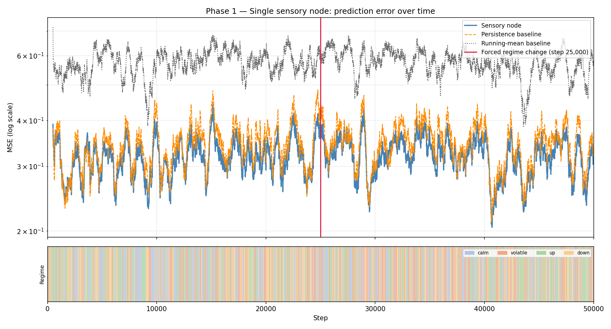
The blue line is the node’s smoothed MSE; orange dashed is the persistence baseline; grey dotted is running mean. The vertical red line marks the forced regime change at step 25,000. Note the spike and recovery — the node detects the shift and adapts. Both baselines spike similarly but the node’s error converges back faster.
Claim 1 is validated. A single predictive coding column can learn useful representations from continuous streaming data and beat naive baselines. ✓
Phase 2: multi-node with ACI (Claim 2, attempt 1)
Now the interesting part. Three sensory nodes — one each for price, volume, and sentiment — plus a model node. InfoNCE loss is applied to align co-temporal ACI projections (same timestep = positive pair). The model node infers the current regime and sends top-down predictions back. I also run standalone “individual” versions of each sensory node with no ACI and no inter-node communication, as the PPI baseline.3
The PPI (Peer Performance Index) measures how much better the collective is than the best individual:
PPI = (individual_energy / collective_energy) - 1
    = (individual_MSE / collective_MSE) - 1
PPI > 0 means the collective is doing better. PPI = 0 means no benefit. PPI < 0 means the collective is somehow worse.
Results after 50,000 steps:
| Stream | Collective MSE | Individual MSE |
|---|---|---|
| Price | 0.3256 | 0.3258 |
| Volume | 0.6944 | 0.6952 |
| Sentiment | 0.2250 | 0.2266 |
| PPI | +0.0021 |
PPI = +0.002. Essentially zero. The collective is essentially tied with the individuals.
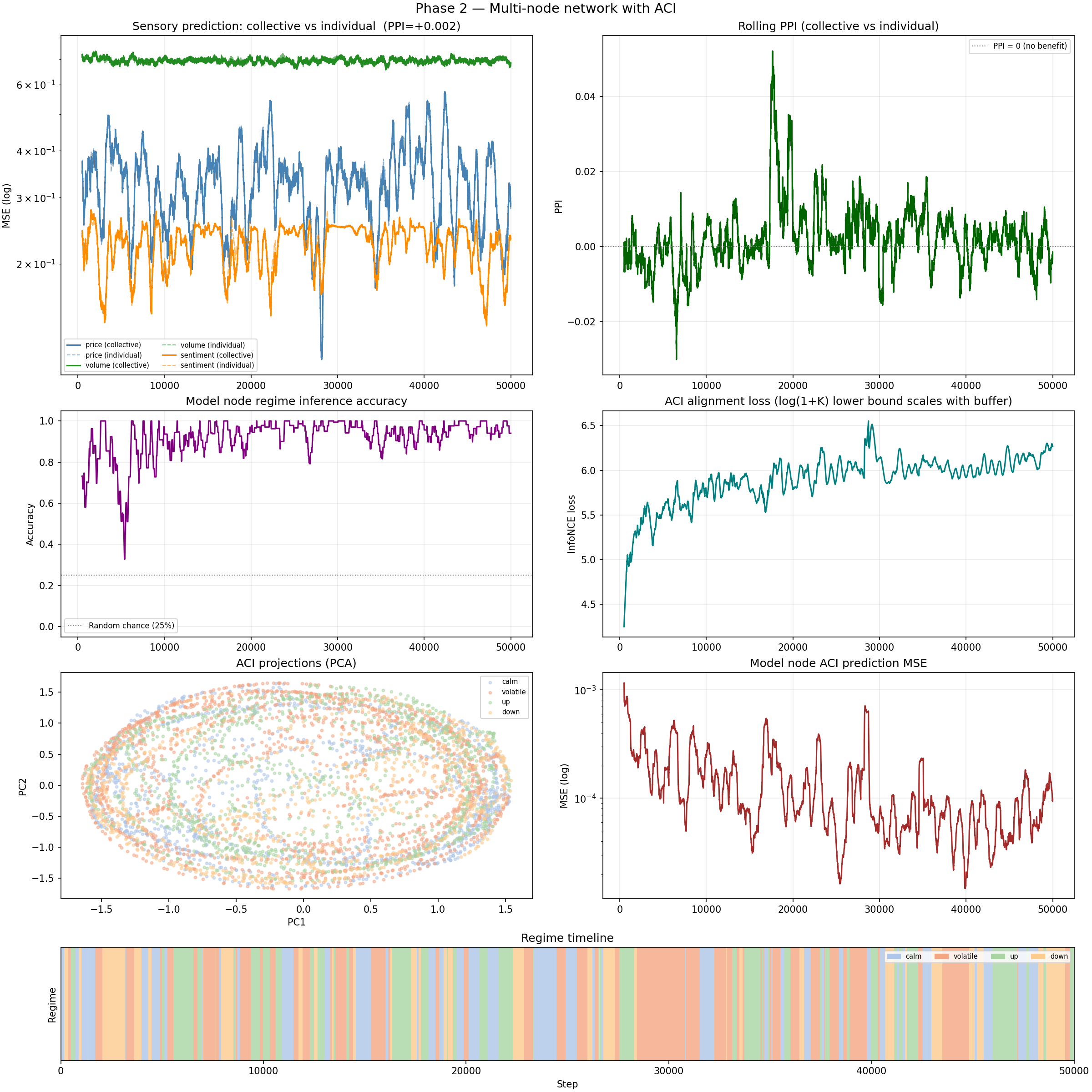
Top left: per-stream MSE curves — collective (solid) and individual (dashed) are nearly identical throughout. Top right: rolling PPI, hovering just above zero. Middle left: regime accuracy — this is 92-96%, which is genuinely impressive. The network understands the regimes. It’s just not using that understanding to improve prediction.
Then I add Phase 2b: lateral voting (sensory nodes exchange regime hypotheses) and top-down predictions (model node tells each sensory node what to expect given the inferred regime). The sensory nodes incorporate this context into their predictions.
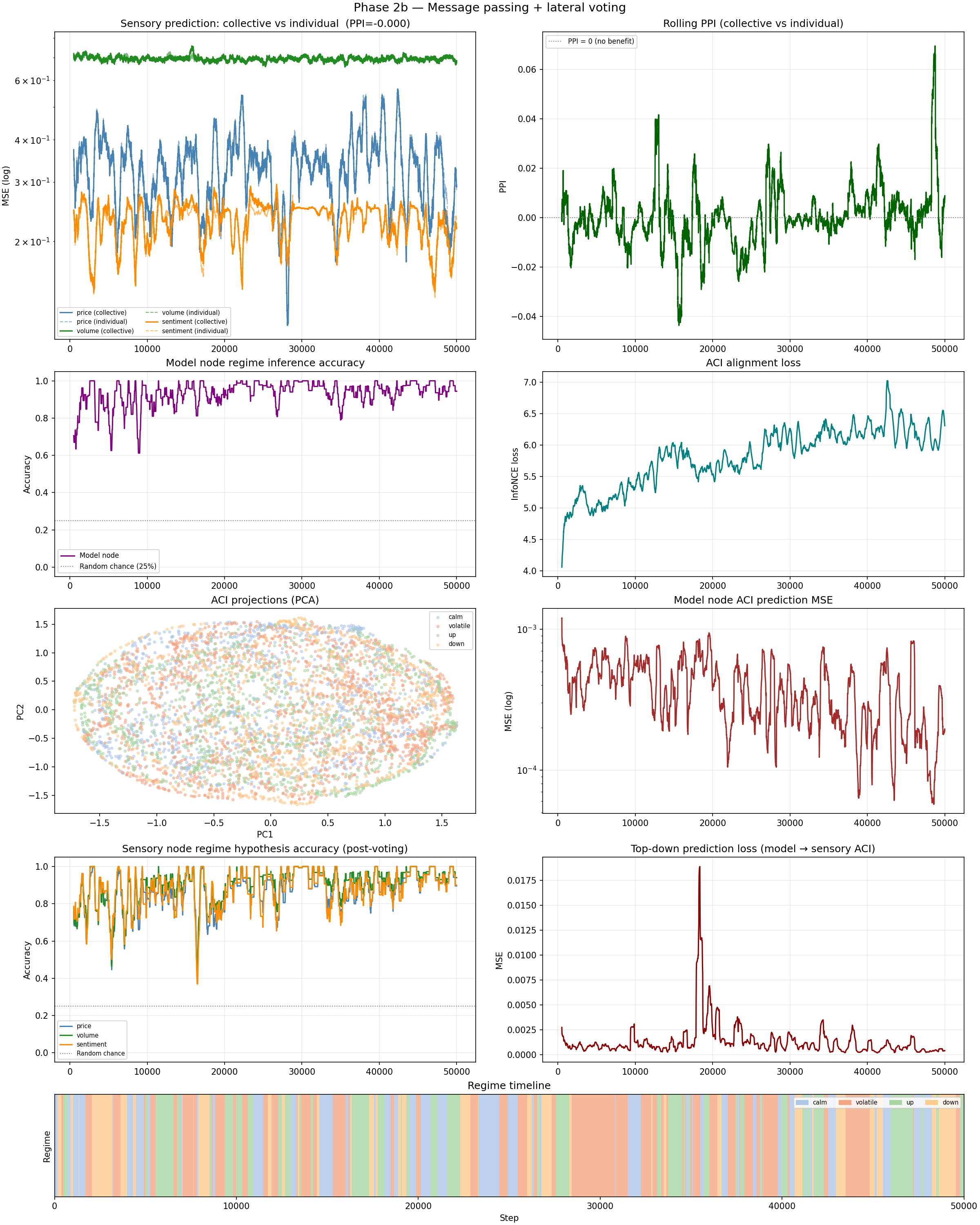
PPI = −0.0000154. It got marginally, if trivially, worse.
The voting mechanism works well — individual node hypothesis accuracy hits 87–91% per stream, meaning each sensory node is correctly inferring the regime most of the time. Regime accuracy at the model node level hits 96%. The collective knows what’s happening. It’s just not translating that knowledge into better predictions.
The diagnosis: InfoNCE needs meaningful co-occurrence
Here’s why it failed, and why the failure is informative rather than just discouraging.
InfoNCE works by finding meaningful co-occurrence. It pulls together representations of things that genuinely should look similar, and pushes apart representations of things that shouldn’t. For CLIP, the structure is obvious: an image of a dog and the caption “a dog” co-occur because they refer to the same thing. For patches of the same image: a wing tile and a fuselage tile co-occur because they’re part of the same airplane.
For our three market streams at the same timestep: co-occurrence doesn’t mean what we want it to mean. At any given step, the fact that the price went up slightly doesn’t tell you much about what the volume did, and vice versa. The streams are correlated through the hidden regime, but that correlation is weak and noisy per timestep — there’s no strong sense in which the price representation at step T “should look like” the volume representation at step T. They’re not fragments of the same thing. They’re projections of the same underlying process through very different observation functions.
So when the InfoNCE loss pushes the price and volume projections together, it’s not finding genuine semantic structure — it’s forcing alignment where no alignment is warranted. The nodes are being penalised for building the specialised, stream-specific representations they actually need. The contrastive signal is noise.
This is a constraint on the approach, not a death sentence. ACI-style contrastive alignment only works when the things you’re aligning are genuinely complementary fragments of a shared underlying reality. The market task doesn’t satisfy this. So let’s find a task that does.
The fix: STL-10 image classification with fragmented input
STL-10 is a standard image classification dataset: 96×96 colour photos across 10 categories (airplane, bird, car, deer, dog, horse, monkey, ship, truck, frog). 5,000 training images, 8,000 test images.
The setup: split each image into N patches. Give one patch to each node. The nodes must classify the image collectively, with each node seeing only its fragment.
96×96 image
┌──────────────────┐
│  node 0  (top)   │  32×96 px  →  CNN encoder  →  ACI projection ─┐
├──────────────────┤                                                  ├→ attention → class [10]
│  node 1  (mid)   │  32×96 px  →  CNN encoder  →  ACI projection ─┤
├──────────────────┤                                                  │
│  node 2  (bot)   │  32×96 px  →  CNN encoder  →  ACI projection ─┘
└──────────────────┘
Now InfoNCE has exactly what it needs. “Node 0’s patch and node 1’s patch are positive pair” means “top third of airplane and middle third of airplane should have similar representations” — which is true, in the sense that both are encoding the same airplane. The co-occurrence is semantically meaningful. Pushing them together in the shared space makes the shared space a map of airplane-ness, not random noise.
Here’s the full image experiment architecture:
flowchart LR
    IMG["96x96 image"]

    subgraph Patches["Patch splitting"]
        PA["Patch 0"]
        PB["Patch 1"]
        PN["Patch N-1"]
    end

    subgraph Encoders["CNN encoders — one per node"]
        EA["Conv x3, Pool, Linear
latent z0"]
        EB["Conv x3, Pool, Linear
latent z1"]
        EN["Conv x3, Pool, Linear
latent zN"]
    end

    subgraph ACIbox["ACI — shared hypersphere"]
        TA(["proj0"])
        TB(["proj1"])
        TN(["projN"])
        NCE["InfoNCE
same image = positive pair
different image = negative"]
    end

    subgraph Head["Collective classifier"]
        ATN["Multi-head self-attention
over N patch tokens"]
        CLS["MLP to 10 classes"]
    end

    IMG --> PA & PB & PN
    PA --> EA --> TA
    PB --> EB --> TB
    PN --> EN --> TN
    TA & TB & TN --> NCE
    TA & TB & TN --> ATN --> CLS
Architecture changes for the image task:
Each node runs a small CNN to encode its patch:
Conv(3→32, 3×3, stride=2) + BatchNorm + ReLU    →  [32, H/2, W/2]
Conv(32→64, 3×3, stride=2) + BatchNorm + ReLU   →  [64, H/4, W/4]
Conv(64→128, 3×3, stride=2) + BatchNorm + ReLU  →  [128, H/8, W/8]
GlobalAveragePool                                →  [128, 1, 1]
flatten → Linear(128→D) → ReLU → Linear(D→D)    →  latent vector [D]
The latent vector goes through the ACI Translator (Linear→ReLU→Linear→L2 normalise) to produce the ACI projection.
The classifier is no longer a simple MLP over concatenated projections. Instead, it uses multi-head self-attention over the patch projections as tokens.4 Each patch is a token; attention learns which patches are informative for which classification decisions. For “airplane” images, the attention head might learn to heavily weight the top patch (sky and wings) while discounting the bottom patch (ground, less distinctive). The architecture:
projections: [B, n_patches, D]  ← one token per node
       ↓
multi-head self-attention (4 heads, D-dim queries/keys/values)
       ↓
residual + LayerNorm
       ↓
mean-pool across patch tokens  →  [B, D]
       ↓
Linear(D→256) → ReLU → Dropout(0.3) → Linear(256→10)
Two PPI metrics are tracked, to separate two different possible sources of improvement:
- PPI_raw: collective vs. independent classifiers. Each individual node has its own CNN encoder trained purely on cross-entropy with no ACI — a fully independent baseline. This measures the total collective advantage, but it’s not entirely fair because the collective also has more parameters.
- PPI_fair: collective vs. linear probes trained on the collective encoder’s latents. Take the shared CNN encoder that was trained with ACI alignment, freeze it, and train a simple linear layer on top — no attention, no multi-node pooling, just one linear layer per patch. If the collective encoder’s latent space is intrinsically better because of ACI alignment, PPI_fair captures that. This is the more meaningful number: it isolates whether the representations themselves improved, not just whether having a bigger classifier helps.
Phase 3: 3 nodes, horizontal strips
50 epochs on STL-10, 3 horizontal strips (32×96 each), batch size 64, cosine annealing LR from 1e-3, InfoNCE weight 0.3.
Final results:
| Accuracy | |
|---|---|
| Collective | 67.9% |
| Best individual (own encoder) | 62.3% |
| Best linear probe (collective encoder) | 58.4% |
| PPI_raw | +9.0% |
| PPI_fair | +16.4% |
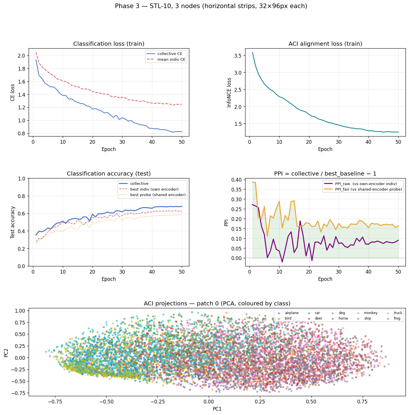
Top left: classification loss curves — collective CE decreases steadily while InfoNCE also decreases (representations aligning). Top right: PPI curves for both metrics, both positive throughout and stabilising after ~30 epochs. Bottom: PCA of the ACI projections from the first node (test set), coloured by class. The classes cluster — the shared space has meaningful geometric structure.
The collective beats the best individual by 9%. But the more telling number is PPI_fair = +16.4%. The linear probes trained on the collective encoder outperform equivalent probes trained on individual node encoders — and both sets of probes are using the same collective encoder, just without multi-node attention. The alignment is making the representations better, not just making the classifier bigger.
Claim 2 is validated on a real task. ✓
Phase 3b: 16 nodes, 4×4 grid
Scale it up. Instead of 3 strips, divide the image into a 4×4 grid of 24×24 pixel tiles. 16 nodes, each seeing 1/16th of the image.
96×96 image → 4×4 grid of 24×24 tiles:
┌────┬────┬────┬────┐
│  0 │  1 │  2 │  3 │  each tile: 24×24 px
├────┼────┼────┼────┤
│  4 │  5 │  6 │  7 │
├────┼────┼────┼────┤
│  8 │  9 │ 10 │ 11 │
├────┼────┼────┼────┤
│ 12 │ 13 │ 14 │ 15 │
└────┴────┴────┴────┘
A 24×24 patch is genuinely tiny. Try to identify a photo category from a random 24×24 square of it — most of the time you’re looking at a patch of sky, or grass, or blurred fur, with no context. If individual nodes can barely do anything useful in isolation, the coordination mechanism has to do all the work.
150 epochs (3× longer to give more nodes time to converge), InfoNCE weight 0.3, max 40 random pairs per step to keep training cost reasonable at C(16,2)=120 possible pairs.
Final results:
| Accuracy | |
|---|---|
| Collective | 72.3% |
| Best individual (own encoder) | 54.4% |
| Best linear probe (collective encoder) | 44.3% |
| PPI_raw | +32.9% |
| PPI_fair | +63.2% |
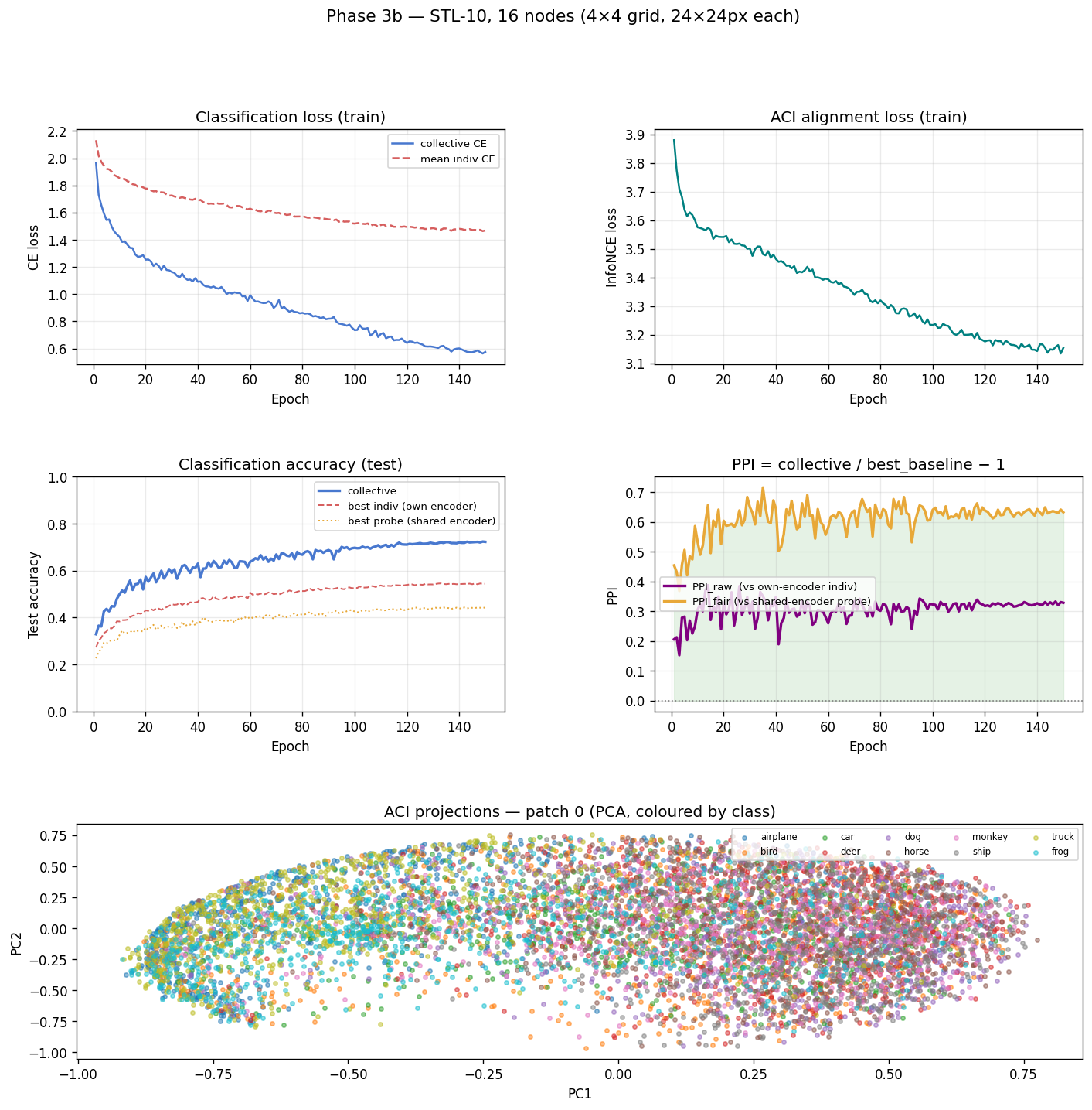
Top left: CE loss declining healthily throughout 150 epochs — no sign of the catastrophic overfitting seen in an earlier unaugmented run. Top right: PPI_raw and PPI_fair both solidly positive and growing. Bottom: PCA of ACI projections from one node — stronger class clustering than Phase 3, because with more positive pairs (16 nodes → 120 pair combinations vs 3 nodes → 3 pairs), the alignment training signal is much richer.
PPI_fair = +63.2%. The collective encoder’s latent space — used with a single linear probe — classifies 63% better than it would without ACI alignment. The representations are fundamentally better shaped because of the contrastive coordination, not just pooled together more cleverly.
Also worth noting: collective accuracy improved from Phase 3 (67.9%) to Phase 3b (72.3%), even though each node now sees far less of the image. More nodes, smaller patches, better collective. The attention head has 16 sources of partial evidence instead of 3. With enough coverage and enough coordination, small patches add up.
Summary
| Phase | Nodes | Task | Collective | Best Individual | PPI_raw | PPI_fair |
|---|---|---|---|---|---|---|
| 1 | 1 | Market price stream | beats baselines ✓ | — | — | — |
| 2 | 3+1 | Market (all streams) | — | — | +0.2% | — |
| 2b | 3+1 | Market + voting | — | — | −0.0% | — |
| 3 | 3 | STL-10, 32×96 strips | 67.9% | 62.3% | +9.0% | +16.4% |
| 3b | 16 | STL-10, 24×24 tiles | 72.3% | 54.4% | +32.9% | +63.2% |
What the numbers mean
The market failure wasn’t just a dead end — it was a diagnostic. Contrastive alignment only works when there’s genuine semantic co-occurrence between what different nodes are processing. Pushing representations together when they have no inherent reason to align destroys specialisation without adding anything useful. The architecture is fine. The task was wrong.
The image results validate the core claim: a collective of partial-view nodes can significantly outperform any individual node, and the benefit grows with fragmentation. When individual nodes are barely better than chance (24×24 patches), the coordination mechanism does all the work — and it does it well.
The PPI_fair / PPI_raw gap is consistent throughout. Roughly half the collective advantage comes from the attention-based multi-node classifier having more information to work with. The other half comes from the representations themselves being intrinsically better after ACI alignment. That’s the part that matters most for the long-term vision — it means the shared space is becoming a real, structured map of the world, not just a technical trick that happens to help one classifier.
This translates to a constraint on where DENDRITE can be usefully deployed: tasks where nodes are observing complementary projections of a shared underlying reality. Images split by patch satisfy this obviously. Sensor arrays monitoring the same physical system satisfy it. Different modalities encoding the same event (audio + video + text description of the same thing) satisfy it strongly. Arbitrary heterogeneous streams that share only a loose statistical correlation over time probably don’t.
What’s next
The next three phases are more interesting architecturally, if harder to implement:
Phase 3 (sleep-wake cycling): Add a fatigue accumulator and a replay buffer. When prediction error accumulates past a threshold, the network “sleeps”: it disconnects from live data, replays its highest-surprise observations (NREM), then runs generative loops on its own internal predictions (REM). Test whether sleeping networks recover faster from regime changes than insomniac networks running continuously.
Phase 4 (active inference): Give the model node an action — it can concentrate its attention on one stream at the cost of degraded sampling on the others. Does active querying (choosing where to look) speed up regime detection compared to passive observation?
Phase 5 (pathological states): Deliberately manipulate the precision ratio — the balance between top-down predictions and bottom-up sensory signals. High ratio: the network hallucinates, ignoring evidence that contradicts its prior. Low ratio: the network becomes purely reactive, chasing noise, losing stable predictions. Does the framework correctly diagnose these states and do the interventions fix them?
There’s also a longer-term question that Phase 3b hints at: the collective accuracy keeps improving with more nodes and smaller patches. At what point does it plateau? And does it plateau at a better level than a single model that sees the whole image? That’s the claim that ultimately matters for a decentralised network — not just “better than any individual node” but “better than a single centralised model.” The experiments so far don’t test that. They’re designed to test whether coordination is possible, not whether it’s optimal. That question is for later.
This article was generated by ChatGPT.
-
Hawkins, Jeff, et al. “A Framework for Intelligence and Cortical Function Based on Grid Cells in the Neocortex.” Frontiers in Neural Circuits 13 (2019). The basic claim is that each cortical column in the neocortex functions as a complete world-model with reference frames, predictions, and voting — not a feature detector feeding a higher area. DENDRITE takes this seriously as an architectural prior. ↩
-
InfoNCE (Noise Contrastive Estimation) loss: given a positive pair (i, j) and a set of N negatives, the loss is −log[exp(sim(i,j)/τ) / Σₖ exp(sim(i,k)/τ)] where sim is cosine similarity and τ is a temperature parameter (0.1 here). Lower temperature = sharper discrimination, harder negatives matter more. The symmetric version averages the loss in both directions. First introduced in van den Oord et al., “Representation Learning with Contrastive Predictive Coding,” 2018. ↩
-
PPI (Peer Performance Index) formula: PPI = (best_individual_metric / collective_metric) − 1. For classification accuracy: PPI = (collective_accuracy / best_individual_accuracy) − 1. Positive means collective outperforms individuals; zero means no benefit; negative means collective underperforms. The “fair” variant uses linear probes on the collective encoder rather than independent encoders as the baseline — this controls for the collective having a larger classifier. ↩
-
Self-attention: given N tokens (here: N patch projections), each token attends to every other token with a learned compatibility score. The output for each token is a weighted sum of all other tokens, where the weights come from the compatibility scores. This lets the classifier dynamically route information — weight the patch tokens that are most relevant for the current classification, downweight uninformative ones. With 4 attention heads, it learns 4 different routing strategies simultaneously. The multi-head variant was introduced in Vaswani et al., “Attention Is All You Need,” 2017. ↩